2. 3. AN INTRODUCTION TO MACHINE LEARNING

Finding the regression line enables the computer to predict the ratings of an item (2) based on the ratings for another item (1). The computer has learned to predict human taste. We are using anthropomorphic terms to describe a process of curve fitting to data. This is the case with all machine learning. It all boils down to applying l techniques from mathematica statistics to find concise mathematical ways to express dependencies between certain kinds of data.

There is no reason to believe that machine learning has any relation to human learning, but the term has stuck. For example, reading machines learn to read after been given samples of each of the letters of the alphabet. Usually they need thousands of samples of each letter in contrast to humans who can learn a new alphabet given only a few examples of each letter. We will return to this issue when we discuss reading machines.

In order to understand machine learning we need to explain how computers make decisions about categorizing objects. To start with, a physical object must be converted into a numerical representation, computers can deal only with numbers. (Actually only with zeros or ones but the conversion of other numbers to binary is automatic.) Sometimes the object is defined by numbers to start with and we will start our discussion with such case.

Suppose we want to have a medical diagnostic computer program that will categorize people as being at risk for a heart attack or not. We may decide to do that on the basis of total cholesterol in the blood and the body mass index (BMI) that gives an indication of whether someone is overweight. It is computed by diving the weight of a person in kilograms by the square of his height in meters and the ideal BMI is 25. Please do not assume that what we describe next has any medical significance. We will use the example only to illustrate machine learning and we are deliberating omitting calibrating the axes. A real diagnostic system must consider more factors. Furthermore the BMI is not a reliable measure of being overweight (see a critique of BMI). Also total cholesterol is not the best indicator, most physicians focus on the low density cholesterol.

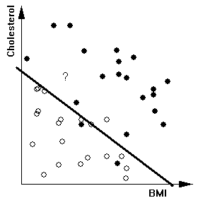
In order to design the diagnostic program we collect data from individuals who had a heart attack and a group who are healthy. Because we deal with only two numbers we can plot them in a graph where the horizontal axis corresponds to the BMI and the vertical axis to the cholesterol. The points on the plane are marked with dark circles for people who had heart attacks and with open circles for the healthy subjects.

Example 1: We can draw a line or another curve to separate the two groups of points and the equivalent computation can be carried out by a computer program. The diagram on the left shows separation by a straight line and the diagram on the right shows separation by part of a polygon (thin lines). When the machine determines a rule for separating the two groups of points we say that the machine has learned to distinguish between the categories. Note that we have not achieved completely separation in either case. The computer can now predict whether a patient is in risk for a heart attack or not. The patient's cholesterol level and BMI determine a point on that plane, for example the one marked with a "?". In this case the computer will decide that the patient is at risk.

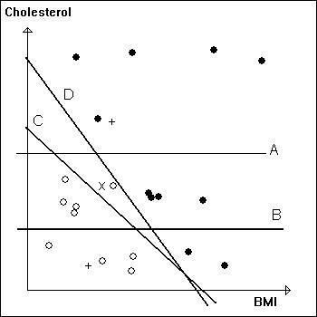
Example 2: We can become ambitious and construct a complicated separating polyline that achieves complete separation. But that is probably more affected by the noise in the data than by any real difference. This is called overfitting and it is likely to fail when the system is asked to classify more data. A better approach is shown on the right where we have drawn two lines. We acknowledge that our system has limitations and we cannot make a reliable decision for data points between the two lines. The plane is separated into three zones indicating "healthy", "uncertain", and "at risk".

We have used a graphical way to describe this simple diagnostic system only for illustration. In a real system the computer calculates a mathematical expression based on the measurements and it determines boundaries so that the expression gives two different values depending on which side of the line (or the polygonal line) a data point is. The parameters of the formula and the separating lines are adjusted until the values of the formula are consistent with the labeling (healthy or heart attack victim).

Example 3: A Mathematical Digression For our example the mathematical expression maybe u*Ch + v*Bm - w where Ch stands for cholesterol and Bm for the BMI. u, v, and w are parameters to be determined during learning. Usually, their initial value can be anything. If we start with u equal to 1, v equal to 0 and w equal to, say, 120 we get the horizontal line marked A on the left given by the equation Ch - 120. For points above the line the expression is positive and for points underneath it, it is negative. Because several points are misclassified the "learning" program may reduce w to, say, 80 producing the line B but that still leaves misclassified points. Setting u to 0.8, v to 8 and w to 288 we obtain the line C that does a better job. The black circle point marked by + may have Ch equal to 130 and Bm equal to 25 and 0.8*130+8*25-288 equals 16. The open circle point marked by + may have Ch equal to 70 and Bm equal to 25 and in this case the expression equals -32, so the results are consistent. However the open circle point marked with x and with Ch equal to 90 and Bm equal to 28 produces the value 1 and that it wrong so the line is modified by decreasing u to 0.6 in which case the expression yields -2. We skip the description of how the computer program modifies the parameters u, v, and w in response to misclassifications. There are well established mathematical methods for doing that and their overall effect is equivalent to modifying the position and orientation of the line.

The important point to keep in mind is that all computer "learning" is equivalent to searching for parameters so that a mathematical expression returns values that are consistent with the classification of the "learning" samples. When a new sample is seen we classify it according to the value returned by the expression. The objects of interest may be described by more than 2 numbers (they usually run to the 100's) and the expressions can be far more complex than what we showed in Example 4 but the deep issues are the same. In particular:

A. Should we use simple expressions and allow for data that we cannot classify or should we use more complex expressions and try to classify everything?

B. How many samples are enough for the learning stage? Clearly the size of the sample has an effect on how hard is the classification problem.

C. Are the object descriptions capturing all that is relevant for the classification task? In our "medical" example we have omitted such variables as genetic predisposition, blood pressure, etc. A practically useful diagnostic system should include all these.

It is appropriate to conclude this section with the observation that some impressive computer programs do not use learning at all. The following is a quote from the article "The making of a chess machine" by Eric J. Lerner. The articles deals with Deep Blue, the chess machine that beat the human world champion. For the full article see
: http://domino.watson.ibm.com/comm/wwwr_thinkresearch.nsf/pages/deepblue296.html

Getting a chess machine to learn from its own mistakes is an appealing idea. It has been tried in the past, but with limited success. ... In contrast, Deep Blue has no learning ability once its values are chosen by its programmers; it carries out exactly the evaluations hardwired into it. So, in any dictionary definition, as well as in the eyes of its creators, Deep Blue has no intelligence at all. That point seemingly got lost in the media discussion of Deep Blue's IQ.

Back to Contents --- Previous Section --- Next Section