MAKING SENSE OUT OF CHAOS
Copyright ©2010 by T. Pavlidis
Summary
Computers have been used to simulate the behavior of large complex systems and, on that basis, used to make predictions. However such predictions are often good only for the short term, weather predictions being the prime example of such a short view. (And, depending on whom you talk, the same is true with stock market predictions.) The term chaos is used to describe systems that are practically unpredictable no matter how much computer power we use. While that is a fascinating theoretical concept, in practical terms chaotic systems are just only at the end of a sequence of systems that are harder and harder to predict.
Section 1 describes a simple system that can exhibit chaotic behavior as well as other forms of complex behavior that are hard to predict, even though in theory are not chaotic. The best way to get an intuitive feeling of what this all means is to try a simulation program that you can download on your computer. Section 2 describes how to download and how to use that program.
If you do not feel comfortable with mathematics or do not want to deal with computer programs you should skip to Section 3 that tries to explain the concept of chaos without resorting to mathematics.
Finally, Section 4 provides a brief discussion of how some scientist have use the mathematical theory of chaos to explain how a deterministic system may exhibit free will.
1. THE FATE OF FISH
A chaotic system is a dynamic where slight variations in the initial conditions result in much larger variations in the output. Weather is a prime example of a chaotic system. Whether it rains today or not it may depend on a minute differences in atmospheric temperature and pressure a few days earlier. This is why accurate long term weather prediction is impossible. (See the Wikipedia article on Lorenz equations http://en.wikipedia.org/wiki/Lorenz_attractor for details on a system of equations used in weather prediction and the peculiar behavior of this equations.)
We must keep in mind that chaotic behavior is a mathematical property of dynamical system and we should read into it any metaphysical implications. While it is hard to make long term predictions about chaotic systems this is also true (albeit to a lesser extent) for most systems of high complexity. I will try to help you develop some intuition about chaotic systems by studying a system whose equation is much simpler than the equations for weather prediction. Here is a simple equation:
x[n+1] = r*x[n]*(1-x[n])
x represents the population of a species of fish as a percentage of the maximum number that its environment can support. n is the generation number and r is a reproduction factor. ('*' stands for multiplication.) The equation can also be written as
xnew = r*x*(1-x)
We replace x by xnew to find the population is subsequent generations, This equation is introduced in page 63 of the book Chaos - Making a New Science by James Gleick [1]. Gleick devotes a whole chapter (pp. 57-80) on a discussion of the chaotic behavior of this equation and credits the theoretical biologist Robert May. Because the equation is non-linear there is no explicit solution expressing x[n] in terms of only n but it is easy to write a program to compute the values of x numerically. The best way to understand chaos (and develop some skepticism about the hype surrounding the concept) is to try different numerical values for r and look at how x varies in generation after generation.
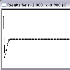
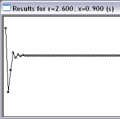
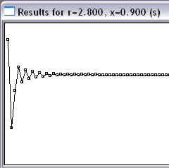
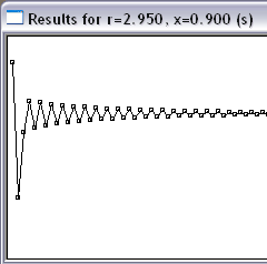
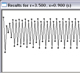
When r is less or equal to 1 (low reproduction rate) the population becomes extinct. When r exceeds 1 but is less than 3 the population reaches eventually a steady state where xnew is the same as x. (Those who still remember their high school math may confirm that the equilibrium value is 1-1/r.) However there is difference in the behavior depending on which side of 2.5 r is. If r less than 2.5 the population reaches the new value gradually, otherwise it fluctuates around it for settling into the equilibrium value. The fluctuations are small and die out as long as r is less than 3, but they become sustained when r exceeds 3.
Figure 1 shows the time plot of x for about
50 generations for different values of r.
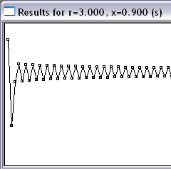
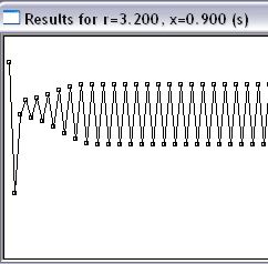
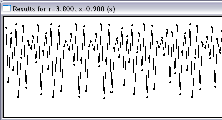
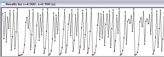
If we increase r even more the fluctuations in the population become increasingly more complicated. For r equal to 3.5 the population fluctuates amongst four possible values and for r equal to 3.8 it fluctuates amongst ten different values. For r equal to 4 we have chaotic behavior. These runs are shown in Figure 2. Figure 3 shows three runs on the same diagram illustrating how minute changes in the initial value of x result eventually in widely different population values.
 |
 |
|
|
||
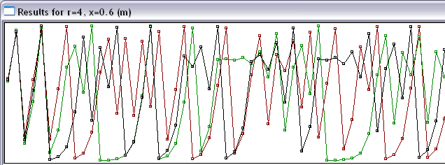
Figure 3: Each color represents one of three runs starting
at x 0.599, 0.600, and 0.601.
You may get a better feeling of how the behavior of the system changes as r changes by running yourselves the program simulating the equations given above.
2. A DEMONSTRATION PROGRAM
You can download the program by clicking
here. (Caveat: The program runs only on Microsoft Windows,
Xp or later.) When you click on the link your browser will warn you that
such files may harm your computer, etc. You should ignore these warnings
if you trust me. (The name of the program is web_mayequ.exe.)
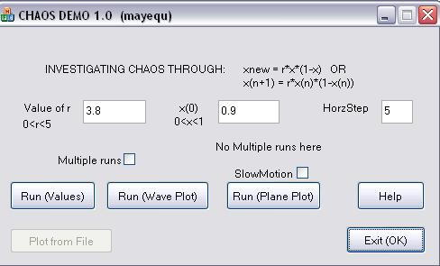
When you run the program you will see a window such as the shown in Figure
4.
|
Figure 4: Simulator
of the dynamics of a fish population. You click one of the first three buttons for a run with different forms of output. |
If you want to see a sampling of the forms of the output click here. "Run (Values)" prints out successive values of x. "Run (Wave Plot)" provides a plot of x in terms of n and the diagrams of Figures 1-3 were made that way. If you check the small box labeled "Multiple Runs" you will get three runs starting for the typed vale of x and two others differing from it by 0.001. This choice will show something different only for values of r close to 4. Figure 3 was made by such a choice.
The entry "HorzStep" determines how stretch out the Wave Plot will be. High values make the results easier to see (especially for multiple runs) but the number of points that fit in the screen goes down.
If you check the "SlowMotion" box, and then you click on "Run (Plane Plot)" you see an animation.
Experiment with different values of r and observe how the output form changes. The program displays only one view at the time to avoid cluttering the computer screen.
3. CHAOS WITHOUT MATHEMATICS
We start with the concept of the continental divide, the mountain ridge (in the Rocky Mountains) that divides the land of the United States in two parts. All rain falling to the west of the divide flows eventually into the Pacific and all falling to the east of the divide flows eventually in the Atlantic (including the Gulf of Mexico). Let us try now to predict the ocean where a particular raindrop will end given its location. If the raindrop is over Ohio the answer is clearly Atlantic or if it is over California the answer is clearly Pacific. If the raindrop is over Colorado we have to know its location with more accuracy in order to predict to which ocean will end up. The closer the raindrop is to the continental divide, the higher the accuracy needed. At some point, when the raindrop is above the ridge itself, we may not be able to make any prediction (even if we take into account minute changes in the wind, temperature, etc) because the required accuracy is beyond our means.
In this example, only a tiny fraction of the rain drops appear to be unpredictable. Consider now Figure 5 where the thick wiggly line represents a continental divide in a (very) roughly drawn map. Not only the continental divide is much longer (so more raindrops will be unpredictable) we also need much higher accuracy for the rest of them in order to predict which ocean will end into. Still, a person looking at the map can tell which parts are part of the Pacific watershed and which are part of the Atlantic watershed.
 |
| Figure 5 |
The example of Figure 6 presents an even more wiggly continental divide. Not only the accuracy needed for predicting the destination of a raindrop has increased but simple inspection is not enough to identify the watersheds. I have placed two colored dots in the figure indicating the destination of two spots. We can also visualize a situation that the continental divide becomes even more wiggly by replacing straight line segments by zigzags. In such a landscape almost all points behave in a chaotic way and we can justifiably call it chaotic. In such a case almost all raindrops will be unpredictable.
You may point that Figure 6 presents a very weird landscape and that we never see such mountain ridges. This is true because the underlying system is quite simple: the position of each drop is described by only two numbers, its longitude and latitude. We say that the system has two degrees of freedom. While chaotic systems with only two degree of freedom are indeed rather contrived, systems with more degrees freedom are almost always chaotic. This is the mathematical discovery of 30 or so years ago that led to the interest in chaos (and a lot of hype as well). While chaotic systems had been known for much longer, they were thought to be peculiarities. Instead they turned out to be the norm rather than the exception for systems with more than two degrees of freedom.
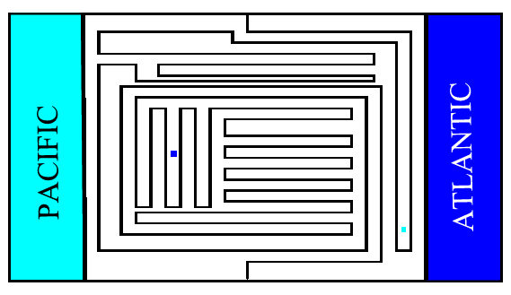 |
| Figure 6 |
4. FREE WILL AND CHAOS
The subject of Free Will has perplexed philosophers for millennia. Both those who believe in an omnipotent and omniscient God as well as atheists who accept a purely mechanical view of the world have trouble with it. The study of "chaos" in the last few decades seems to provide a way out of the old paradoxes. In his 1987 book [1] James Gleick quotes Doyne Farmer (p. 251) saying "... (chaos) struck me as an operational way to define free will, in a way that allowed you to reconcile free will with determinism. The system is deterministic, but you can't say what it's going to do next." Edward Wilson provides a solid analysis of connection between free will and chaos in at least one of his books [2]. In addition, there has been a plethora of articles on the web by several authors, both in the context of science (Paul Davies, Linas Vepstas, etc) and of religion (Rabbi Winston, Marc Perkel, etc). Unfortunately there has been a lot of hype on the significance of chaos (even Gleick's book suffers from that) and the quality of the web postings varies widely, from solid scientific to hyped-up "New Age." Amongst recent writers Matt Ridley [3] looks for an alternate explanation for free will but I found it rather unconvincing and, in essence, based on a special case of chaos.
If we think of the process by which a human being makes a decision we may realize that it involves many variables, genetic predisposition, cultural background, education, perception of the environment and the intentions of others, etc. Even when we view the process as purely mechanical it is likely to be chaotic and therefore to have an unpredictable outcome. Is unpredictability of action the same as free will? Not necessarily, but from a practical viewpoint it appears the same way to an outside observer. If such an observer cannot predict how you will act in a given situation, then he/she may assume that you have free will.
One might argue that chaos provides the illusion of free will rather than free will. Wilson [2] supplies two counter-arguments. One is that "Free will as a side product of illusion would seem to be free will enough to drive human progress and offer happiness." The other is a bit more complex (and I promised to keep this essay simple) but the key phrase is "Because the individual mind cannot be fully known and predicted, the self can go on ... believing in its own free will. ... in every operational sense that applies to the knowable self, the mind does have free will." (Emphasis in the original.)
Notes
Sections 3 and 4 are based on an essay Free Will and Chaos that I posted on my web site in 2006. Link to Slides from a talk based on that essay.
Works CIted
- James Gleick, Chaos - Making a New Science, New York, Viking, 1987.
- Edward Wilson, Consilience - The Unity of Knowledge, New York, Vintage, 1998, pp. 130-132.
- Matt Ridley, Nature via Nurture, New York, Harper Collins, 2003, pp. 272-275.
First Posted: June 26, 2010 — Latest Update: June 28, 2010